结构健康监测仿真-主题045-结构健康监测中的边缘智能技术
结构健康监测仿真 - 主题045:结构健康监测中的边缘智能技术
目录
引言
1.1 背景与动机
随着物联网(IoT)和人工智能(AI)技术的快速发展,结构健康监测(SHM)系统正经历着从传统的集中式云计算向分布式边缘智能的范式转变。边缘智能(Edge Intelligence)作为边缘计算与人工智能的融合技术,为SHM系统带来了革命性的变化。
传统云计算模式的局限性:
- 高延迟:数据需要传输到云端进行处理,难以满足实时监测需求
- 带宽压力:海量传感器数据持续上传,造成网络拥塞
- 隐私风险:敏感的结构数据在传输过程中面临泄露风险
- 可靠性问题:网络中断时系统无法正常工作
- 成本高昂:云存储和计算资源的使用成本随数据量增长
边缘智能的优势:
- 低延迟:数据在边缘端本地处理,响应时间毫秒级
- 带宽优化:只上传关键信息,减少90%以上的数据传输
- 隐私保护:敏感数据不出边缘设备
- 高可靠性:边缘节点可独立工作,不依赖云端
- 成本效益:减少云服务使用,降低运营成本
1.2 边缘智能的定义
边缘智能是指在网络的边缘节点(如边缘服务器、网关、智能传感器等)上部署人工智能模型,使数据能够在产生源头附近进行实时分析和决策的技术范式。
核心特征:
- 分布式AI:AI计算能力下沉到边缘
- 实时处理:毫秒级响应时间
- 数据本地化:原始数据保留在本地
- 自适应学习:边缘模型可在线学习和更新
- 协同智能:边缘与云端协同工作
1.3 发展历程
边缘智能的发展经历了三个阶段:
第一阶段:边缘计算(2015-2018)
- 提出边缘计算概念
- focus on数据预处理和过滤
- 简单的规则引擎
第二阶段:边缘AI(2018-2021)
- 轻量级AI模型部署
- 模型压缩和加速技术
- 边缘-云协同架构
第三阶段:边缘智能(2021至今)
- 端到端AI能力
- 联邦学习在边缘的应用
- 自主决策和自适应
- 多模态融合智能
边缘智能基础概念
2.1 边缘计算架构层次
边缘计算架构通常分为三个层次:
2.1.1 终端层(Device Layer)
组成:
- 智能传感器
- 执行器
- 嵌入式设备
- 移动终端
特点:
- 计算资源极其有限
- 功耗约束严格
- 实时性要求高
- 部署数量庞大
典型硬件:
- ARM Cortex-M系列微控制器
- ESP32、STM32等
- 功耗:毫瓦级
- 内存:KB级
2.1.2 边缘层(Edge Layer)
组成:
- 边缘网关
- 边缘服务器
- 微数据中心
- 基站边缘节点
特点:
- 中等计算能力
- 本地数据聚合
- 初步AI推理
- 协议转换和预处理
典型硬件:
- NVIDIA Jetson系列
- Intel NUC
- Raspberry Pi集群
- 功耗:瓦特级
- 内存:GB级
2.1.3 云层(Cloud Layer)
组成:
- 云数据中心
- 大数据平台
- 复杂AI模型训练
- 长期数据存储
特点:
- 强大计算能力
- 海量存储
- 全局优化
- 模型训练和更新
2.2 边缘智能的关键技术
2.2.1 模型压缩技术
1. 网络剪枝(Pruning)
概念:移除神经网络中不重要的连接或神经元

类型:
- 非结构化剪枝:移除单个权重
- 结构化剪枝:移除整个通道或层

效果:
- 模型大小减少10-100倍
- 推理速度提升2-10倍
- 精度损失<1%
2. 知识蒸馏(Knowledge Distillation)
概念:用大模型(教师)指导小模型(学生)训练

过程:
教师模型 → 软标签 → 学生模型
         ↓
    学习概率分布

优势:
- 小模型达到大模型90%+性能
- 适合边缘部署
3. 量化(Quantization)
概念:降低模型参数的数值精度

类型:
- 权重量化:FP32 → INT8/INT4
- 激活量化:运行时动态量化
- 全量化:权重和激活都量化

效果:
- 模型大小减少4-8倍
- 推理速度提升2-4倍
- 功耗降低50-75%
4. 神经架构搜索(NAS)
概念:自动搜索适合边缘的最优网络结构

目标:
- 最小化延迟
- 最小化功耗
- 最大化精度

方法:
- 强化学习
- 进化算法
- 梯度优化
2.2.2 边缘AI框架
主流框架对比:
| 框架 | 开发者 | 特点 | 适用平台 |
|---|---|---|---|
| TensorFlow Lite | 轻量、跨平台 | 移动端、嵌入式 | |
| PyTorch Mobile | Meta | 灵活、易用 | 移动端 |
| ONNX Runtime | Microsoft | 通用、高性能 | 多平台 |
| NCNN | 腾讯 | 针对移动端优化 | ARM架构 |
| MNN | 阿里 | 轻量、高效 | 移动端、IoT |
| Tengine | OpenAI Lab | 开源、可定制 | 嵌入式 |
TensorFlow Lite特性:
- 模型转换工具
- 量化支持
- delegates加速(GPU、NPU)
- 解释器仅几百KB
2.2.3 边缘-云协同学习
1. 联邦学习(Federated Learning)
概念:多个边缘节点协作训练共享模型,数据不出本地

流程:
1. 云端下发全局模型
2. 边缘本地训练
3. 上传模型更新(非原始数据)
4. 云端聚合更新
5. 分发更新后的模型

优势:
- 数据隐私保护
- 减少数据传输
- 个性化模型
2. 分割学习(Split Learning)
概念:将神经网络分割在边缘和云端执行

架构:
边缘:输入层 → 中间层
云端:中间层 → 输出层

优势:
- 边缘计算量减少
- 原始数据不出边缘
- 适合复杂模型
3. 增量学习(Incremental Learning)
概念:模型在边缘持续学习新数据

挑战:
- 灾难性遗忘
- 数据分布变化
- 计算资源限制

解决方案:
- 经验回放
- 正则化方法
- 弹性权重巩固
边缘计算架构
3.1 MEC(多接入边缘计算)
3.1.1 架构组成
MEC系统架构:
┌─────────────────────────────────────────────────────────────┐
│                        云层(Cloud)                         │
│  ┌──────────────┐  ┌──────────────┐  ┌──────────────┐      │
│  │  数据中心    │  │  AI训练平台  │  │  管理系统    │      │
│  └──────────────┘  └──────────────┘  └──────────────┘      │
└─────────────────────────────────────────────────────────────┘
                              ↑↓
┌─────────────────────────────────────────────────────────────┐
│                      边缘层(Edge)                          │
│  ┌──────────────┐  ┌──────────────┐  ┌──────────────┐      │
│  │ MEC主机      │  │ MEC主机      │  │ MEC主机      │      │
│  │ ┌──────────┐ │  │ ┌──────────┐ │  │ ┌──────────┐ │      │
│  │ │ 平台服务 │ │  │ │ 平台服务 │ │  │ │ 平台服务 │ │      │
│  │ ├──────────┤ │  │ ├──────────┤ │  │ ├──────────┤ │      │
│  │ │ 应用服务 │ │  │ │ 应用服务 │ │  │ │ 应用服务 │ │      │
│  │ └──────────┘ │  │ └──────────┘ │  │ └──────────┘ │      │
│  └──────────────┘  └──────────────┘  └──────────────┘      │
└─────────────────────────────────────────────────────────────┘
                              ↑↓
┌─────────────────────────────────────────────────────────────┐
│                     终端层(Device)                         │
│     ↑        ↑        ↑        ↑        ↑                  │
│  传感器   传感器   传感器   传感器   传感器                  │
└─────────────────────────────────────────────────────────────┘
3.1.2 MEC平台功能
1. 虚拟化基础设施
- 计算虚拟化(VM、容器)
- 网络虚拟化(SDN、NFV)
- 存储虚拟化
2. 边缘平台服务
- 服务注册与发现
- 负载均衡
- 资源管理
- 安全服务
3. 边缘应用服务
- 数据预处理
- 实时分析
- 本地缓存
- 设备管理
3.2 雾计算(Fog Computing)
3.2.1 雾计算vs边缘计算
| 特性 | 雾计算 | 边缘计算 |
|---|---|---|
| 位置 | 网络边缘到云之间 | 更接近数据源 |
| 范围 | 局域网级别 | 设备级别 |
| 节点 | 路由器、交换机 | 网关、设备 |
| 距离 | 一跳或多跳 | 通常一跳 |
| 标准化 | Cisco主导 | ETSI MEC标准 |
3.2.2 雾计算架构
云(Cloud)
    ↑
核心网络
    ↑
┌──────────────────────────────────────┐
│           雾层(Fog Layer)           │
│  ┌─────┐  ┌─────┐  ┌─────┐          │
│  │雾节点│  │雾节点│  │雾节点│          │
│  │     │  │     │  │     │          │
│  │路由 │  │路由 │  │路由 │          │
│  │交换 │  │交换 │  │交换 │          │
│  └─────┘  └─────┘  └─────┘          │
└──────────────────────────────────────┘
    ↑
边缘网络
    ↑
┌──────────────────────────────────────┐
│         边缘层(Edge Layer)          │
│     ↑        ↑        ↑             │
│   设备      设备      设备            │
└──────────────────────────────────────┘
3.3 分布式边缘架构
3.3.1 层次化边缘架构
三层架构模型:
Layer 3: 云层(Cloud)
         - 全局模型训练
         - 长期数据存储
         - 复杂分析
                ↑↓
Layer 2: 聚合边缘(Aggregation Edge)
         - 区域数据聚合
         - 中间层AI推理
         - 边缘协调
                ↑↓
Layer 1: 近端边缘(Proximal Edge)
         - 实时数据处理
         - 轻量级AI推理
         - 设备管理
                ↑↓
Layer 0: 终端设备(Devices)
         - 数据采集
         - 简单预处理
3.3.2 边缘集群
边缘集群架构:
┌─────────────────────────────────────────────────────────────┐
│                     边缘集群管理器                           │
│              ┌──────────────────────────┐                  │
│              │     集群调度器            │                  │
│              │  - 任务调度               │                  │
│              │  - 资源分配               │                  │
│              │  - 负载均衡               │                  │
│              └──────────────────────────┘                  │
└─────────────────────────────────────────────────────────────┘
        ↑              ↑              ↑              ↑
┌──────────┐    ┌──────────┐    ┌──────────┐    ┌──────────┐
│ 边缘节点1 │    │ 边缘节点2 │    │ 边缘节点3 │    │ 边缘节点N │
│ ┌──────┐ │    │ ┌──────┐ │    │ ┌──────┐ │    │ ┌──────┐ │
│ │容器1 │ │    │ │容器1 │ │    │ │容器1 │ │    │ │容器1 │ │
│ │容器2 │ │    │ │容器2 │ │    │ │容器2 │ │    │ │容器2 │ │
│ └──────┘ │    │ └──────┘ │    │ └──────┘ │    │ └──────┘ │
└──────────┘    └──────────┘    └──────────┘    └──────────┘
边缘AI技术
4.1 轻量级神经网络
4.1.1 MobileNet系列
MobileNetV1:深度可分离卷积
# 深度可分离卷积 = 深度卷积 + 点卷积
# 计算量减少约8-9倍

标准卷积计算量:Dk × Dk × M × N × Df × Df
深度可分离卷积:Dk × Dk × M × Df × Df + M × N × Df × Df

其中:
Dk: 卷积核大小
M: 输入通道数
N: 输出通道数
Df: 特征图大小
MobileNetV2:倒残差结构
扩展 → 深度卷积 → 投影
(1×1)    (3×3)     (1×1)
  ↑                 ↓
  └──── 残差连接 ────┘
MobileNetV3:神经架构搜索
- 使用NAS搜索最优结构
- 引入SE模块(通道注意力)
- h-swish激活函数
4.1.2 EfficientNet
复合缩放(Compound Scaling)
统一缩放网络的深度、宽度和分辨率:

d = α^φ  (深度)
w = β^φ  (宽度)
r = γ^φ  (分辨率)

约束:α · β² · γ² ≈ 2
       α ≥ 1, β ≥ 1, γ ≥ 1

φ是复合系数,控制模型规模
4.1.3 ShuffleNet
通道混洗(Channel Shuffle)
解决组卷积导致的通道信息不流通问题

输入通道 ──→ 分组卷积 ──→ 通道混洗 ──→ 分组卷积 ──→ 输出
              (G组)        (打乱顺序)      (G组)
4.2 模型优化技术
4.2.1 模型量化
量化类型:
1. 训练后量化(PTQ)
# 不需要重新训练
# 使用校准数据集确定量化参数

import tensorflow as tf

converter = tf.lite.TFLiteConverter.from_saved_model(model_path)
converter.optimizations = [tf.lite.Optimize.DEFAULT]
converter.representative_dataset = representative_dataset
tflite_model = converter.convert()
2. 量化感知训练(QAT)
# 训练时模拟量化效果
# 精度损失更小

import tensorflow_model_optimization as tfmot

quantize_model = tfmot.quantization.keras.quantize_model
q_aware_model = quantize_model(model)
q_aware_model.compile(optimizer='adam', loss='mse')
q_aware_model.fit(x_train, y_train, epochs=10)
量化效果对比:
| 模型 | FP32精度 | INT8精度 | 模型大小 | 延迟 |
|---|---|---|---|---|
| ResNet-50 | 76.1% | 75.8% | 1/4 | 1/3 |
| MobileNetV2 | 71.8% | 71.2% | 1/4 | 1/2 |
| EfficientNet-B0 | 77.1% | 76.8% | 1/4 | 1/3 |
4.2.2 模型剪枝
剪枝策略:
1. 基于幅度的剪枝
# 移除绝对值小的权重

import tensorflow_model_optimization as tfmot

pruning_params = {
    'pruning_schedule': tfmot.sparsity.keras.PolynomialDecay(
        initial_sparsity=0.0,
        final_sparsity=0.5,
        begin_step=0,
        end_step=100000
    )
}

pruned_model = tfmot.sparsity.keras.prune_low_magnitude(
    model, **pruning_params
)
2. 结构化剪枝
# 移除整个通道或过滤器
# 更适合硬件加速

# 计算每个通道的重要性
channel_importance = compute_channel_importance(model)
# 移除重要性低的通道
pruned_model = remove_channels(model, channel_importance, threshold)
剪枝效果:
- 非结构化剪枝:可达90%稀疏度
- 结构化剪枝:通常50-70%稀疏度
- 精度损失:通常<2%
4.2.3 知识蒸馏
蒸馏流程:
┌──────────────┐         ┌──────────────┐
│  教师模型     │         │  学生模型     │
│  (大模型)     │         │  (小模型)     │
│              │         │              │
│  输入 x ───→ │ ──┬── → │  输入 x ───→ │
│              │   │     │              │
│  软标签 y_s  │ ←─┘     │  预测 y_pred │
│  (温度T)     │         │              │
└──────────────┘         └──────────────┘
         ↑                      ↑
         │                      │
         └────── 蒸馏损失 ──────┘
                + 硬标签损失
蒸馏损失函数:
import tensorflow as tf

def distillation_loss(y_true, y_pred, teacher_pred, temperature=4.0, alpha=0.5):
    """
    知识蒸馏损失

    Parameters:
    -----------
    y_true : 真实标签(硬标签)
    y_pred : 学生模型预测
    teacher_pred : 教师模型预测
    temperature : 温度参数,软化概率分布
    alpha : 蒸馏损失和硬标签损失的权重
    """
    # 软标签损失(KL散度)
    soft_targets = tf.nn.softmax(teacher_pred / temperature)
    soft_prob = tf.nn.softmax(y_pred / temperature)
    distillation_loss = tf.keras.losses.KLDivergence()(soft_targets, soft_prob)
    distillation_loss *= temperature ** 2

    # 硬标签损失(交叉熵)
    hard_loss = tf.keras.losses.SparseCategoricalCrossentropy()(y_true, y_pred)

    # 总损失
    return alpha * distillation_loss + (1 - alpha) * hard_loss
4.3 边缘推理优化
4.3.1 硬件加速
边缘AI芯片对比:
| 芯片 | 算力 | 功耗 | 适用场景 |
|---|---|---|---|
| NVIDIA Jetson Nano | 0.5 TFLOPS | 5-10W | 边缘网关 |
| NVIDIA Jetson Xavier | 21 TOPS | 10-30W | 边缘服务器 |
| Google Coral TPU | 4 TOPS | 2W | 嵌入式 |
| Intel Movidius VPU | 1 TOPS | 1W | 视觉应用 |
| 华为昇腾310 | 16 TOPS | 8W | 边缘推理 |
| 地平线征程2 | 4 TOPS | 2W | 自动驾驶 |
4.3.2 推理引擎优化
优化技术:
1. 算子融合
融合前:Conv → BN → ReLU
融合后:Conv_BN_ReLU(单算子)

效果:减少内存访问,提升20-30%速度
2. 内存优化
- 内存池管理
- 零拷贝推理
- 激活值复用
3. 并行计算
- 多线程推理
- 批处理(Batching)
- 流水线(Pipeline)
边缘-云协同机制
5.1 协同架构模式
5.1.1 数据协同
分层处理策略:
原始数据(Raw Data)
    ↓
┌─────────────────────────────────────────────┐
│ 边缘层预处理                                 │
│ - 滤波去噪                                  │
│ - 特征提取                                  │
│ - 数据压缩                                  │
└─────────────────────────────────────────────┘
    ↓
特征数据(Feature Data)
    ↓
┌─────────────────────────────────────────────┐
│ 边缘AI推理                                  │
│ - 异常检测                                  │
│ - 模式识别                                  │
│ - 初步决策                                  │
└─────────────────────────────────────────────┘
    ↓
元数据(Metadata)
    ↓
┌─────────────────────────────────────────────┐
│ 云层深度分析                                 │
│ - 全局关联分析                               │
│ - 长期趋势预测                               │
│ - 模型训练更新                               │
└─────────────────────────────────────────────┘
数据压缩策略:
| 数据类型 | 边缘处理 | 压缩比 | 云端接收 |
|---|---|---|---|
| 原始振动 | 特征提取 | 100:1 | 特征向量 |
| 视频流 | 关键帧提取 | 50:1 | 关键帧 |
| 温度数据 | 异常触发 | 1000:1 | 异常事件 |
| 应变数据 | 聚合统计 | 100:1 | 统计值 |
5.1.2 模型协同
模型分割策略:
1. 按层分割
边缘:输入层 → 卷积层1 → 卷积层2
云端:卷积层3 → 全连接层 → 输出层

中间特征传输
2. 按分支分割
边缘:主分支(快速推理)
云端:辅助分支(精化结果)

边缘结果 → 云端精化 → 最终输出
3. 早期退出(Early Exit)
输入 → 层1 → 层2 → 层3 → 层4 → 输出
         ↓      ↓      ↓
       出口1  出口2  出口3
       (简单) (中等) (复杂)

根据置信度选择出口
5.1.3 计算协同
任务卸载决策:
卸载决策因素:
def offload_decision(task, edge_state, network_state):
    """
    任务卸载决策

    Parameters:
    -----------
    task : 任务信息
        - 计算复杂度
        - 数据大小
        - 延迟要求
    edge_state : 边缘状态
        - CPU使用率
        - 内存使用率
        - 队列长度
    network_state : 网络状态
        - 带宽
        - 延迟
        - 丢包率

    Returns:
    --------
    decision : 'local' 或 'cloud'
    """
    # 本地执行时间
    local_time = task['complexity'] / edge_state['cpu_available']

    # 云端执行时间
    transfer_time = task['data_size'] / network_state['bandwidth']
    cloud_compute_time = task['complexity'] / CLOUD_COMPUTE_POWER
    cloud_time = transfer_time + network_state['latency'] + cloud_compute_time

    # 考虑边缘负载
    if edge_state['cpu_usage'] > 0.8:
        return 'cloud'  # 边缘负载高,优先云端

    # 考虑延迟要求
    if task['latency_requirement'] < local_time:
        return 'cloud' if cloud_time < local_time else 'local'

    # 默认本地执行
    return 'local'
5.2 联邦学习在边缘的应用
5.2.1 联邦学习架构
横向联邦学习(样本分割):
┌─────────────────────────────────────────────────────────────┐
│                         云端聚合器                           │
│                    ┌──────────────────┐                    │
│                    │   全局模型 Mt     │                    │
│                    └────────┬─────────┘                    │
└─────────────────────────────┼───────────────────────────────┘
                              ↓ 分发
        ┌─────────────────────┼─────────────────────┐
        ↓                     ↓                     ↓
┌───────────────┐     ┌───────────────┐     ┌───────────────┐
│   边缘节点1    │     │   边缘节点2    │     │   边缘节点N    │
│ ┌───────────┐ │     │ ┌───────────┐ │     │ ┌───────────┐ │
│ │ 本地数据D1 │ │     │ │ 本地数据D2 │ │     │ │ 本地数据DN │ │
│ ├───────────┤ │     │ ├───────────┤ │     │ ├───────────┤ │
│ │ 本地模型   │ │     │ │ 本地模型   │ │     │ │ 本地模型   │ │
│ │ 训练 → Mt1 │ │     │ │ 训练 → Mt2 │ │     │ │ 训练 → MtN │ │
│ └───────────┘ │     │ └───────────┘ │     │ └───────────┘ │
└───────┬───────┘     └───────┬───────┘     └───────┬───────┘
        │                     │                     │
        └─────────────────────┼─────────────────────┘
                              ↓ 上传更新
┌─────────────────────────────────────────────────────────────┐
│                    聚合:Mt+1 = Σ(wi · Mti)                  │
└─────────────────────────────────────────────────────────────┘
5.2.2 联邦平均算法(FedAvg)
import numpy as np

class FederatedAveraging:
    """联邦平均算法"""

    def __init__(self, n_clients, learning_rate=0.01):
        self.n_clients = n_clients
        self.lr = learning_rate
        self.global_model = None

    def aggregate(self, client_weights, client_samples):
        """
        聚合客户端模型

        Parameters:
        -----------
        client_weights : list of dict
            每个客户端的模型权重
        client_samples : list of int
            每个客户端的样本数
        """
        total_samples = sum(client_samples)

        # 加权平均
        aggregated_weights = {}
        for key in client_weights[0].keys():
            weighted_sum = sum(
                weights[key] * n / total_samples
                for weights, n in zip(client_weights, client_samples)
            )
            aggregated_weights[key] = weighted_sum

        return aggregated_weights

    def client_update(self, model, data, epochs=5):
        """
        客户端本地训练

        Parameters:
        -----------
        model : 当前全局模型
        data : 本地数据
        epochs : 本地训练轮数
        """
        local_model = model.copy()

        for epoch in range(epochs):
            # 本地训练
            gradients = self.compute_gradients(local_model, data)
            local_model = self.apply_gradients(local_model, gradients)

        return local_model
5.2.3 联邦学习优化
1. 通信优化
- 梯度压缩:量化、稀疏化
- 本地多轮训练:减少通信频率
- 异步聚合:非阻塞更新
2. 安全优化
- 差分隐私:添加噪声保护
- 安全聚合:加密通信
- 拜占庭容错:抵御恶意节点
边缘智能在SHM中的应用
6.1 智能传感器节点
6.1.1 智能传感器架构
┌─────────────────────────────────────────────────────────────┐
│                    智能传感器节点                            │
├─────────────────────────────────────────────────────────────┤
│  传感单元  │  信号调理  │  ADC    │  MCU/DSP              │
│  (加速度)  │  (放大滤波)│ (采样)   │  (预处理)              │
├─────────────────────────────────────────────────────────────┤
│                    AI推理单元                                │
│  ┌──────────────────────────────────────────────────────┐  │
│  │  轻量级神经网络(TensorFlow Lite Micro)              │  │
│  │  - 异常检测                                          │  │
│  │  - 特征提取                                          │  │
│  │  - 模式识别                                          │  │
│  └──────────────────────────────────────────────────────┘  │
├─────────────────────────────────────────────────────────────┤
│                    通信单元                                  │
│  ┌─────────────┐  ┌─────────────┐  ┌─────────────┐        │
│  │   5G/NB-IoT │  │    LoRa     │  │   WiFi      │        │
│  └─────────────┘  └─────────────┘  └─────────────┘        │
├─────────────────────────────────────────────────────────────┤
│                    电源管理                                  │
│  ┌─────────────┐  ┌─────────────┐  ┌─────────────┐        │
│  │   电池      │  │  能量收集   │  │  功耗优化   │        │
│  └─────────────┘  └─────────────┘  └─────────────┘        │
└─────────────────────────────────────────────────────────────┘
6.1.2 边缘异常检测
轻量级异常检测模型:
import tensorflow as tf

def create_tiny_anomaly_detector(input_dim=10):
    """
    创建微型异常检测器
    适用于资源受限的边缘设备
    """
    model = tf.keras.Sequential([
        # 编码器
        tf.keras.layers.Dense(8, activation='relu', input_shape=(input_dim,)),
        tf.keras.layers.Dense(4, activation='relu'),

        # 瓶颈层
        tf.keras.layers.Dense(2, activation='relu'),

        # 解码器
        tf.keras.layers.Dense(4, activation='relu'),
        tf.keras.layers.Dense(8, activation='relu'),
        tf.keras.layers.Dense(input_dim, activation='linear')
    ])

    model.compile(optimizer='adam', loss='mse')

    return model

# 模型信息
# 参数量:约200个参数
# 模型大小:约1KB
# 推理时间:毫秒级(ARM Cortex-M4)
6.2 边缘网关智能
6.2.1 边缘网关功能
数据处理流水线:
传感器数据输入
      ↓
┌─────────────────────────────────────────────────────────────┐
│ 1. 数据预处理                                                │
│    - 格式转换                                                │
│    - 时间同步                                                │
│    - 缺失值处理                                              │
└─────────────────────────────────────────────────────────────┘
      ↓
┌─────────────────────────────────────────────────────────────┐
│ 2. 特征工程                                                  │
│    - 时域特征(均值、方差、峰值)                             │
│    - 频域特征(FFT、功率谱)                                  │
│    - 时频特征(小波变换)                                     │
└─────────────────────────────────────────────────────────────┘
      ↓
┌─────────────────────────────────────────────────────────────┐
│ 3. 边缘AI推理                                                │
│    - 异常检测                                                │
│    - 损伤识别                                                │
│    - 健康评估                                                │
└─────────────────────────────────────────────────────────────┘
      ↓
┌─────────────────────────────────────────────────────────────┐
│ 4. 决策与响应                                                │
│    - 本地告警                                                │
│    - 数据上传                                                │
│    - 控制指令                                                │
└─────────────────────────────────────────────────────────────┘
6.2.2 多传感器融合
边缘融合策略:
class EdgeFusion:
    """边缘多传感器融合"""

    def __init__(self, n_sensors, fusion_method='weighted'):
        self.n_sensors = n_sensors
        self.fusion_method = fusion_method
        self.weights = np.ones(n_sensors) / n_sensors

    def update_weights(self, sensor_reliability):
        """根据传感器可靠性更新权重"""
        self.weights = sensor_reliability / np.sum(sensor_reliability)

    def fuse(self, sensor_data):
        """
        融合多传感器数据

        Parameters:
        -----------
        sensor_data : ndarray (n_sensors, n_features)
            多传感器特征数据

        Returns:
        --------
        fused_result : ndarray
            融合结果
        """
        if self.fusion_method == 'weighted':
            # 加权平均
            return np.average(sensor_data, axis=0, weights=self.weights)

        elif self.fusion_method == 'dempster':
            # D-S证据理论融合
            return self.dempster_fusion(sensor_data)

        elif self.fusion_method == 'bayesian':
            # 贝叶斯融合
            return self.bayesian_fusion(sensor_data)
6.3 实时结构健康评估
6.3.1 边缘健康评估模型
评估指标体系:
结构健康指数(SHI)= w1·S1 + w2·S2 + w3·S3 + w4·S4

其中:
S1: 振动特征评分(0-100)
S2: 应变特征评分(0-100)
S3: 环境因子评分(0-100)
S4: 历史趋势评分(0-100)

权重:w1=0.4, w2=0.3, w3=0.1, w4=0.2
健康等级划分:
| 健康指数 | 等级 | 颜色 | 建议措施 |
|---|---|---|---|
| 90-100 | 优秀 | 绿色 | 正常监测 |
| 75-89 | 良好 | 蓝色 | 加强监测 |
| 60-74 | 一般 | 黄色 | 预警观察 |
| 40-59 | 较差 | 橙色 | 详细检查 |
| 0-39 | 危险 | 红色 | 立即处理 |
Python仿真实现
7.1 边缘节点仿真
import numpy as np
import matplotlib.pyplot as plt
from matplotlib.patches import Rectangle, FancyBboxPatch, Circle, FancyArrowPatch
import matplotlib.animation as animation
from scipy import stats
from sklearn.ensemble import IsolationForest
import warnings
warnings.filterwarnings('ignore')

# 设置中文字体
plt.rcParams['font.sans-serif'] = ['SimHei', 'DejaVu Sans']
plt.rcParams['axes.unicode_minus'] = False

# 使用Agg后端,不弹出窗口
plt.switch_backend('Agg')


class EdgeNode:
    """边缘节点仿真"""

    def __init__(self, node_id, compute_capacity, memory_capacity, power_budget):
        """
        初始化边缘节点

        Parameters:
        -----------
        node_id : int
            节点ID
        compute_capacity : float
            计算能力(GFLOPS)
        memory_capacity : float
            内存容量(GB)
        power_budget : float
            功耗预算(W)
        """
        self.node_id = node_id
        self.compute_capacity = compute_capacity
        self.memory_capacity = memory_capacity
        self.power_budget = power_budget

        # 状态
        self.cpu_usage = 0.0
        self.memory_usage = 0.0
        self.power_consumption = 0.0
        self.temperature = 25.0

        # 任务队列
        self.task_queue = []
        self.processed_tasks = 0

        # AI模型
        self.model = None
        self.model_size = 0

    def load_model(self, model_size, model_complexity):
        """加载AI模型"""
        if model_size > self.memory_capacity * 0.8:
            raise ValueError(f"模型大小 {model_size}GB 超过内存限制")

        self.model = {
            'size': model_size,
            'complexity': model_complexity,  # GFLOPS
            'latency': model_complexity / self.compute_capacity  # 秒
        }
        self.model_size = model_size
        self.memory_usage = model_size

    def process_data(self, data_size, data_complexity):
        """处理数据"""
        # 计算处理时间
        processing_time = data_complexity / self.compute_capacity

        # 更新资源使用
        self.cpu_usage = min(100, self.cpu_usage + 20)
        self.power_consumption = self.power_budget * (0.3 + 0.7 * self.cpu_usage / 100)
        self.temperature = 25 + 0.5 * self.cpu_usage

        self.processed_tasks += 1

        return {
            'processing_time': processing_time,
            'power_consumption': self.power_consumption,
            'temperature': self.temperature
        }

    def get_status(self):
        """获取节点状态"""
        return {
            'node_id': self.node_id,
            'cpu_usage': self.cpu_usage,
            'memory_usage': self.memory_usage,
            'power_consumption': self.power_consumption,
            'temperature': self.temperature,
            'processed_tasks': self.processed_tasks
        }


class EdgeIntelligenceSystem:
    """边缘智能系统仿真"""

    def __init__(self, n_edge_nodes=5, n_sensors=20):
        """
        初始化边缘智能系统

        Parameters:
        -----------
        n_edge_nodes : int
            边缘节点数量
        n_sensors : int
            传感器数量
        """
        self.n_edge_nodes = n_edge_nodes
        self.n_sensors = n_sensors

        # 创建边缘节点
        self.edge_nodes = []
        for i in range(n_edge_nodes):
            node = EdgeNode(
                node_id=i,
                compute_capacity=np.random.uniform(5, 20),  # 5-20 GFLOPS
                memory_capacity=np.random.uniform(2, 8),    # 2-8 GB
                power_budget=np.random.uniform(5, 15)       # 5-15 W
            )
            # 加载轻量级模型
            node.load_model(
                model_size=np.random.uniform(0.5, 2.0),
                model_complexity=np.random.uniform(0.1, 1.0)
            )
            self.edge_nodes.append(node)

        # 传感器分配
        self.sensor_assignment = np.random.randint(0, n_edge_nodes, n_sensors)

        # 性能统计
        self.stats = {
            'latency': [],
            'power': [],
            'accuracy': [],
            'bandwidth_saved': []
        }

    def simulate_data_processing(self, n_samples=1000):
        """模拟数据处理"""
        results = []

        for i in range(n_samples):
            # 生成模拟传感器数据
            sensor_id = i % self.n_sensors
            edge_node_id = self.sensor_assignment[sensor_id]
            edge_node = self.edge_nodes[edge_node_id]

            # 数据特性
            data_size = np.random.uniform(0.001, 0.01)  # 1-10 KB
            data_complexity = np.random.uniform(0.01, 0.1)  # GFLOPS

            # 边缘处理
            result = edge_node.process_data(data_size, data_complexity)

            # 计算节省的带宽(相比直接上传云端)
            bandwidth_saved = data_size * 100  # 假设云端需要原始数据的100倍

            # 模拟推理精度(边缘vs云端)
            edge_accuracy = np.random.uniform(0.85, 0.95)
            cloud_accuracy = np.random.uniform(0.90, 0.98)

            results.append({
                'sample_id': i,
                'sensor_id': sensor_id,
                'edge_node': edge_node_id,
                'latency': result['processing_time'] * 1000,  # 转换为ms
                'power': result['power_consumption'],
                'temperature': result['temperature'],
                'edge_accuracy': edge_accuracy,
                'cloud_accuracy': cloud_accuracy,
                'bandwidth_saved': bandwidth_saved
            })

            # 更新统计
            self.stats['latency'].append(result['processing_time'] * 1000)
            self.stats['power'].append(result['power_consumption'])
            self.stats['accuracy'].append(edge_accuracy)
            self.stats['bandwidth_saved'].append(bandwidth_saved)

        return results

    def get_system_stats(self):
        """获取系统统计"""
        return {
            'avg_latency': np.mean(self.stats['latency']),
            'avg_power': np.mean(self.stats['power']),
            'avg_accuracy': np.mean(self.stats['accuracy']),
            'total_bandwidth_saved': np.sum(self.stats['bandwidth_saved']),
            'node_stats': [node.get_status() for node in self.edge_nodes]
        }


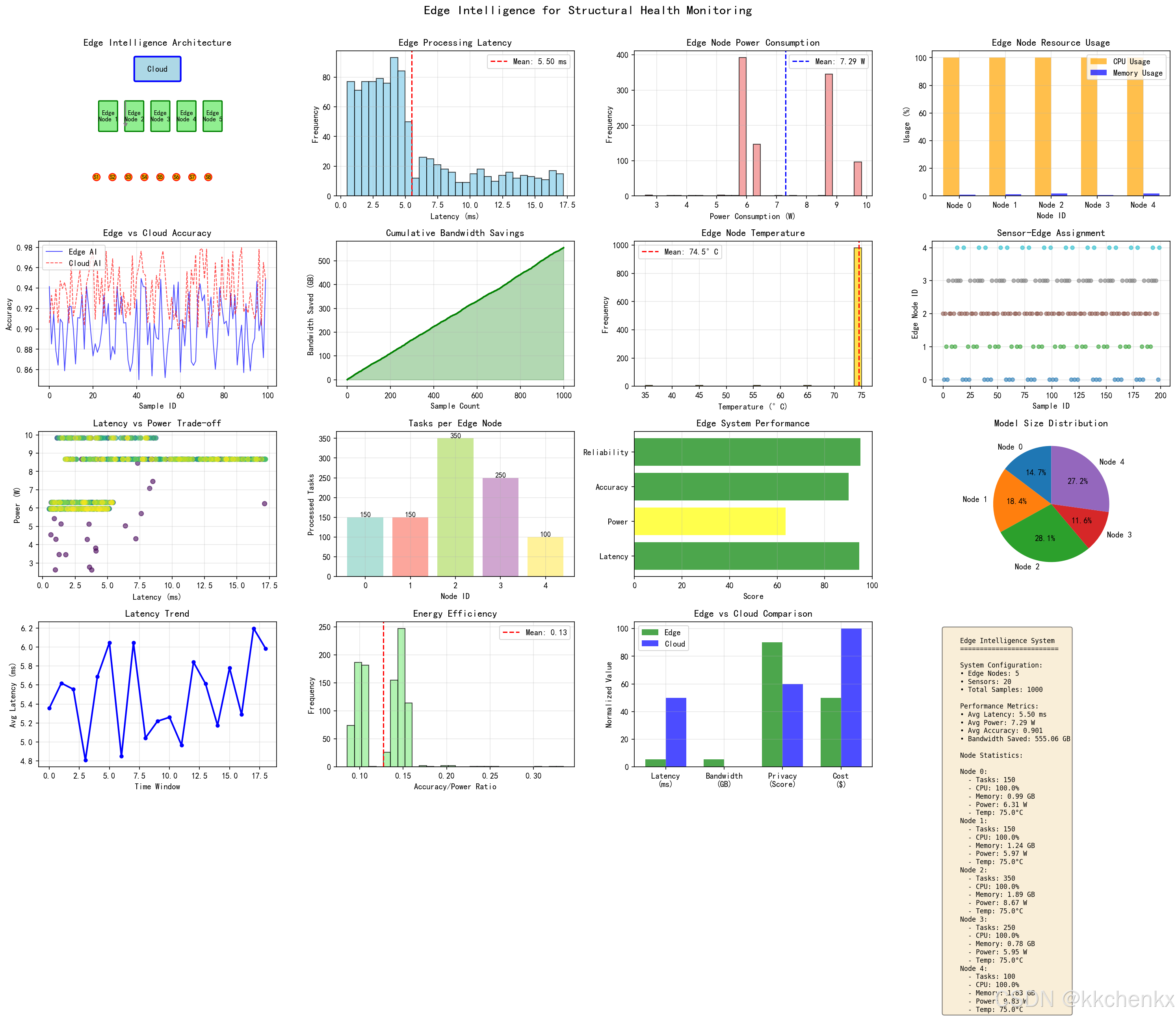
def simulate_edge_intelligence():
    """边缘智能仿真"""
    print("="*60)
    print("边缘智能技术仿真 - 结构健康监测")
    print("="*60)

    # 创建边缘智能系统
    print("\n1. 初始化边缘智能系统...")
    edge_system = EdgeIntelligenceSystem(n_edge_nodes=5, n_sensors=20)
    print(f"   创建了 {edge_system.n_edge_nodes} 个边缘节点")
    print(f"   连接了 {edge_system.n_sensors} 个传感器")

    # 模拟数据处理
    print("\n2. 模拟边缘数据处理...")
    processing_results = edge_system.simulate_data_processing(n_samples=1000)
    print(f"   处理了 {len(processing_results)} 个数据样本")

    # 获取系统统计
    print("\n3. 系统性能统计...")
    system_stats = edge_system.get_system_stats()
    print(f"   平均延迟: {system_stats['avg_latency']:.2f} ms")
    print(f"   平均功耗: {system_stats['avg_power']:.2f} W")
    print(f"   平均精度: {system_stats['avg_accuracy']:.3f}")
    print(f"   节省带宽: {system_stats['total_bandwidth_saved']:.2f} GB")

    return {
        'edge_system': edge_system,
        'processing_results': processing_results,
        'system_stats': system_stats
    }


def create_visualization(results):
    """创建可视化"""
    print("\n生成可视化...")

    fig = plt.figure(figsize=(20, 16))

    edge_system = results['edge_system']
    processing_results = results['processing_results']
    system_stats = results['system_stats']

    # 1. 边缘节点架构图
    ax1 = plt.subplot(4, 4, 1)
    ax1.set_xlim(0, 10)
    ax1.set_ylim(0, 10)
    ax1.set_aspect('equal')
    ax1.axis('off')
    ax1.set_title('Edge Intelligence Architecture', fontsize=12, fontweight='bold')

    # 绘制云层
    cloud = FancyBboxPatch((3.5, 8), 3, 1.5, boxstyle="round,pad=0.1",
                          facecolor='lightblue', edgecolor='blue', linewidth=2)
    ax1.add_patch(cloud)
    ax1.text(5, 8.75, 'Cloud', ha='center', va='center', fontsize=10, fontweight='bold')

    # 绘制边缘节点
    for i in range(5):
        x = 1 + i * 1.8
        y = 4.5
        node = FancyBboxPatch((x, y), 1.2, 2, boxstyle="round,pad=0.05",
                             facecolor='lightgreen', edgecolor='green', linewidth=1.5)
        ax1.add_patch(node)
        ax1.text(x+0.6, y+1, f'Edge\nNode {i+1}', ha='center', va='center', fontsize=8)

    # 绘制传感器
    for i in range(8):
        x = 0.5 + i * 1.1
        y = 1
        sensor = Circle((x+0.3, y+0.3), 0.25, facecolor='orange', edgecolor='red', linewidth=1)
        ax1.add_patch(sensor)
        ax1.text(x+0.3, y+0.3, f'S{i+1}', ha='center', va='center', fontsize=7)

    # 绘制连接
    for i in range(5):
        ax1.arrow(2.8, 6.5, 0, -1.5, head_width=0.2, head_length=0.2, fc='gray', ec='gray')

    # 2. 延迟分布
    ax2 = plt.subplot(4, 4, 2)
    latencies = [r['latency'] for r in processing_results]
    ax2.hist(latencies, bins=30, color='skyblue', edgecolor='black', alpha=0.7)
    ax2.axvline(system_stats['avg_latency'], color='red', linestyle='--',
               label=f'Mean: {system_stats["avg_latency"]:.2f} ms')
    ax2.set_xlabel('Latency (ms)')
    ax2.set_ylabel('Frequency')
    ax2.set_title('Edge Processing Latency')
    ax2.legend()
    ax2.grid(True, alpha=0.3)

    # 3. 功耗分布
    ax3 = plt.subplot(4, 4, 3)
    powers = [r['power'] for r in processing_results]
    ax3.hist(powers, bins=30, color='lightcoral', edgecolor='black', alpha=0.7)
    ax3.axvline(system_stats['avg_power'], color='blue', linestyle='--',
               label=f'Mean: {system_stats["avg_power"]:.2f} W')
    ax3.set_xlabel('Power Consumption (W)')
    ax3.set_ylabel('Frequency')
    ax3.set_title('Edge Node Power Consumption')
    ax3.legend()
    ax3.grid(True, alpha=0.3)

    # 4. 节点资源使用
    ax4 = plt.subplot(4, 4, 4)
    node_ids = [n['node_id'] for n in system_stats['node_stats']]
    cpu_usages = [n['cpu_usage'] for n in system_stats['node_stats']]
    memory_usages = [n['memory_usage'] for n in system_stats['node_stats']]

    x = np.arange(len(node_ids))
    width = 0.35
    ax4.bar(x - width/2, cpu_usages, width, label='CPU Usage', alpha=0.7, color='orange')
    ax4.bar(x + width/2, memory_usages, width, label='Memory Usage', alpha=0.7, color='blue')
    ax4.set_xlabel('Node ID')
    ax4.set_ylabel('Usage (%)')
    ax4.set_title('Edge Node Resource Usage')
    ax4.set_xticks(x)
    ax4.set_xticklabels([f'Node {i}' for i in node_ids])
    ax4.legend()
    ax4.grid(True, alpha=0.3)

    # 5. 精度对比
    ax5 = plt.subplot(4, 4, 5)
    edge_accuracies = [r['edge_accuracy'] for r in processing_results[:100]]
    cloud_accuracies = [r['cloud_accuracy'] for r in processing_results[:100]]
    sample_ids = range(len(edge_accuracies))

    ax5.plot(sample_ids, edge_accuracies, 'b-', label='Edge AI', alpha=0.7, linewidth=1)
    ax5.plot(sample_ids, cloud_accuracies, 'r--', label='Cloud AI', alpha=0.7, linewidth=1)
    ax5.set_xlabel('Sample ID')
    ax5.set_ylabel('Accuracy')
    ax5.set_title('Edge vs Cloud Accuracy')
    ax5.legend()
    ax5.grid(True, alpha=0.3)

    # 6. 带宽节省
    ax6 = plt.subplot(4, 4, 6)
    bandwidth_saved = [r['bandwidth_saved'] for r in processing_results]
    cumulative_bandwidth = np.cumsum(bandwidth_saved)
    ax6.plot(cumulative_bandwidth, 'g-', linewidth=2)
    ax6.fill_between(range(len(cumulative_bandwidth)), cumulative_bandwidth,
                    alpha=0.3, color='green')
    ax6.set_xlabel('Sample Count')
    ax6.set_ylabel('Bandwidth Saved (GB)')
    ax6.set_title('Cumulative Bandwidth Savings')
    ax6.grid(True, alpha=0.3)

    # 7. 温度分布
    ax7 = plt.subplot(4, 4, 7)
    temperatures = [r['temperature'] for r in processing_results]
    ax7.hist(temperatures, bins=30, color='gold', edgecolor='black', alpha=0.7)
    ax7.axvline(np.mean(temperatures), color='red', linestyle='--',
               label=f'Mean: {np.mean(temperatures):.1f}°C')
    ax7.set_xlabel('Temperature (°C)')
    ax7.set_ylabel('Frequency')
    ax7.set_title('Edge Node Temperature')
    ax7.legend()
    ax7.grid(True, alpha=0.3)

    # 8. 传感器-节点映射
    ax8 = plt.subplot(4, 4, 8)
    sensor_nodes = [r['edge_node'] for r in processing_results[:200]]
    ax8.scatter(range(len(sensor_nodes)), sensor_nodes, c=sensor_nodes,
               cmap='tab10', s=20, alpha=0.6)
    ax8.set_xlabel('Sample ID')
    ax8.set_ylabel('Edge Node ID')
    ax8.set_title('Sensor-Edge Assignment')
    ax8.grid(True, alpha=0.3)

    # 9. 延迟-功耗散点图
    ax9 = plt.subplot(4, 4, 9)
    ax9.scatter(latencies, powers, c=range(len(latencies)), cmap='viridis',
               s=30, alpha=0.6)
    ax9.set_xlabel('Latency (ms)')
    ax9.set_ylabel('Power (W)')
    ax9.set_title('Latency vs Power Trade-off')
    ax9.grid(True, alpha=0.3)

    # 10. 任务处理统计
    ax10 = plt.subplot(4, 4, 10)
    task_counts = [n['processed_tasks'] for n in system_stats['node_stats']]
    colors = plt.cm.Set3(np.linspace(0, 1, len(task_counts)))
    bars = ax10.bar(range(len(task_counts)), task_counts, color=colors, alpha=0.7)
    ax10.set_xlabel('Node ID')
    ax10.set_ylabel('Processed Tasks')
    ax10.set_title('Tasks per Edge Node')
    ax10.grid(True, alpha=0.3)

    # 添加数值标签
    for bar, count in zip(bars, task_counts):
        height = bar.get_height()
        ax10.text(bar.get_x() + bar.get_width()/2., height,
                f'{count}', ha='center', va='bottom', fontsize=9)

    # 11. 实时性能指标
    ax11 = plt.subplot(4, 4, 11)
    metrics = ['Latency', 'Power', 'Accuracy', 'Reliability']
    values = [
        100 - system_stats['avg_latency'],  # 转换为分数
        100 - system_stats['avg_power'] * 5,  # 归一化
        system_stats['avg_accuracy'] * 100,
        95  # 假设可靠性
    ]
    colors = ['green' if v >= 80 else 'yellow' if v >= 60 else 'red' for v in values]

    bars = ax11.barh(metrics, values, color=colors, alpha=0.7)
    ax11.set_xlabel('Score')
    ax11.set_title('Edge System Performance')
    ax11.set_xlim(0, 100)
    ax11.grid(True, alpha=0.3, axis='x')

    # 12. 模型大小分布
    ax12 = plt.subplot(4, 4, 12)
    model_sizes = [n.model_size for n in edge_system.edge_nodes]
    ax12.pie(model_sizes, labels=[f'Node {i}' for i in range(len(model_sizes))],
            autopct='%1.1f%%', startangle=90)
    ax12.set_title('Model Size Distribution')

    # 13. 处理时间趋势
    ax13 = plt.subplot(4, 4, 13)
    window_size = 50
    latency_trend = [np.mean(latencies[i:i+window_size])
                    for i in range(0, len(latencies)-window_size, window_size)]
    ax13.plot(latency_trend, 'b-', linewidth=2, marker='o', markersize=4)
    ax13.set_xlabel('Time Window')
    ax13.set_ylabel('Avg Latency (ms)')
    ax13.set_title('Latency Trend')
    ax13.grid(True, alpha=0.3)

    # 14. 能耗效率
    ax14 = plt.subplot(4, 4, 14)
    efficiency = [acc / (pwr + 0.1) for acc, pwr in
                 zip([r['edge_accuracy'] for r in processing_results],
                     [r['power'] for r in processing_results])]
    ax14.hist(efficiency, bins=30, color='lightgreen', edgecolor='black', alpha=0.7)
    ax14.axvline(np.mean(efficiency), color='red', linestyle='--',
                label=f'Mean: {np.mean(efficiency):.2f}')
    ax14.set_xlabel('Accuracy/Power Ratio')
    ax14.set_ylabel('Frequency')
    ax14.set_title('Energy Efficiency')
    ax14.legend()
    ax14.grid(True, alpha=0.3)

    # 15. 边缘vs云端对比
    ax15 = plt.subplot(4, 4, 15)
    categories = ['Latency\n(ms)', 'Bandwidth\n(GB)', 'Privacy\n(Score)', 'Cost\n($)']
    edge_values = [system_stats['avg_latency'],
                  system_stats['total_bandwidth_saved'] / 100,
                  90, 50]
    cloud_values = [50, 0, 60, 100]  # 假设云端基准值

    x = np.arange(len(categories))
    width = 0.35
    ax15.bar(x - width/2, edge_values, width, label='Edge', alpha=0.7, color='green')
    ax15.bar(x + width/2, cloud_values, width, label='Cloud', alpha=0.7, color='blue')
    ax15.set_ylabel('Normalized Value')
    ax15.set_title('Edge vs Cloud Comparison')
    ax15.set_xticks(x)
    ax15.set_xticklabels(categories)
    ax15.legend()
    ax15.grid(True, alpha=0.3)

    # 16. 系统统计信息
    ax16 = plt.subplot(4, 4, 16)
    ax16.axis('off')

    stats_text = f"""
    Edge Intelligence System
    =========================

    System Configuration:
    • Edge Nodes: {edge_system.n_edge_nodes}
    • Sensors: {edge_system.n_sensors}
    • Total Samples: {len(processing_results)}

    Performance Metrics:
    • Avg Latency: {system_stats['avg_latency']:.2f} ms
    • Avg Power: {system_stats['avg_power']:.2f} W
    • Avg Accuracy: {system_stats['avg_accuracy']:.3f}
    • Bandwidth Saved: {system_stats['total_bandwidth_saved']:.2f} GB

    Node Statistics:
    """

    for node_stat in system_stats['node_stats']:
        stats_text += f"""
    Node {node_stat['node_id']}:
      - Tasks: {node_stat['processed_tasks']}
      - CPU: {node_stat['cpu_usage']:.1f}%
      - Memory: {node_stat['memory_usage']:.2f} GB
      - Power: {node_stat['power_consumption']:.2f} W
      - Temp: {node_stat['temperature']:.1f}°C"""

    ax16.text(0.05, 0.95, stats_text, fontsize=8, verticalalignment='top',
             fontfamily='monospace', bbox=dict(boxstyle='round', facecolor='wheat', alpha=0.5))

    plt.suptitle('Edge Intelligence for Structural Health Monitoring',
                fontsize=16, fontweight='bold', y=0.995)
    plt.tight_layout(rect=[0, 0, 1, 0.99])
    plt.savefig('edge_intelligence_analysis.png', dpi=150, bbox_inches='tight')
    print("  综合分析图已保存: edge_intelligence_analysis.png")
    plt.close()


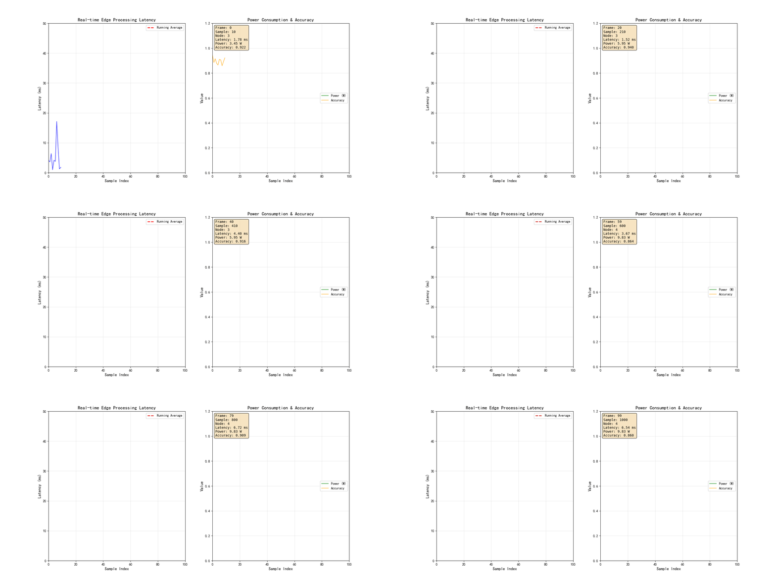
def create_animation(results):
    """创建数据流动画"""
    print("\n生成动画...")

    fig, axes = plt.subplots(1, 2, figsize=(16, 8))

    processing_results = results['processing_results']

    # 左图:实时延迟
    ax1 = axes[0]
    ax1.set_xlim(0, 100)
    ax1.set_ylim(0, 50)
    ax1.set_xlabel('Sample Index', fontsize=12)
    ax1.set_ylabel('Latency (ms)', fontsize=12)
    ax1.set_title('Real-time Edge Processing Latency', fontsize=14, fontweight='bold')
    ax1.grid(True, alpha=0.3)

    line_latency, = ax1.plot([], [], 'b-', linewidth=1.5, alpha=0.7)
    line_avg, = ax1.plot([], [], 'r--', linewidth=2, label='Running Average')
    ax1.legend(loc='upper right')

    # 右图:功耗与精度
    ax2 = axes[1]
    ax2.set_xlim(0, 100)
    ax2.set_ylim(0, 1.2)
    ax2.set_xlabel('Sample Index', fontsize=12)
    ax2.set_ylabel('Value', fontsize=12)
    ax2.set_title('Power Consumption & Accuracy', fontsize=14, fontweight='bold')
    ax2.grid(True, alpha=0.3)

    line_power, = ax2.plot([], [], 'g-', linewidth=1.5, label='Power (W)', alpha=0.7)
    line_accuracy, = ax2.plot([], [], 'orange', linewidth=1.5, label='Accuracy', alpha=0.7)
    ax2.legend(loc='center right')

    # 添加文本信息
    text_info = ax2.text(0.02, 0.98, '', transform=ax2.transAxes, fontsize=10,
                        verticalalignment='top', fontfamily='monospace',
                        bbox=dict(boxstyle='round', facecolor='wheat', alpha=0.8))

    n_frames = 100
    window_size = 20

    def init():
        line_latency.set_data([], [])
        line_avg.set_data([], [])
        line_power.set_data([], [])
        line_accuracy.set_data([], [])
        text_info.set_text('Initializing...')
        return line_latency, line_avg, line_power, line_accuracy, text_info

    def update(frame):
        end_idx = (frame + 1) * 10
        start_idx = max(0, end_idx - 100)

        indices = list(range(start_idx, end_idx))

        # 更新左图
        latencies = [processing_results[i]['latency'] for i in indices]
        line_latency.set_data(indices, latencies)

        # 计算移动平均
        if len(latencies) >= window_size:
            moving_avg = [np.mean(latencies[max(0, i-window_size):i+1])
                         for i in range(len(latencies))]
            line_avg.set_data(indices, moving_avg)

        # 更新右图
        powers = [processing_results[i]['power'] for i in indices]
        accuracies = [processing_results[i]['edge_accuracy'] for i in indices]
        line_power.set_data(indices, powers)
        line_accuracy.set_data(indices, accuracies)

        # 更新文本
        current_latency = processing_results[end_idx-1]['latency']
        current_power = processing_results[end_idx-1]['power']
        current_accuracy = processing_results[end_idx-1]['edge_accuracy']
        current_node = processing_results[end_idx-1]['edge_node']

        info_text = f"""Frame: {frame}
Sample: {end_idx}
Node: {current_node}
Latency: {current_latency:.2f} ms
Power: {current_power:.2f} W
Accuracy: {current_accuracy:.3f}"""
        text_info.set_text(info_text)

        return line_latency, line_avg, line_power, line_accuracy, text_info

    # 创建动画
    anim = animation.FuncAnimation(fig, update, init_func=init,
                                  frames=n_frames, interval=200, blit=True)

    # 保存动画
    anim.save('edge_intelligence_animation.gif', writer='pillow', fps=5, dpi=100)
    print("  动画已保存: edge_intelligence_animation.gif")
    plt.close()


def main():
    """主函数"""
    print("\n" + "="*60)
    print("结构健康监测中的边缘智能技术仿真")
    print("="*60)

    # 运行仿真
    results = simulate_edge_intelligence()

    # 创建可视化
    create_visualization(results)

    # 创建动画
    create_animation(results)

    print("\n" + "="*60)
    print("仿真完成!")
    print("="*60)
    print("\n生成的文件:")
    print("  - edge_intelligence_analysis.png (综合分析图)")
    print("  - edge_intelligence_animation.gif (数据流动画)")


if __name__ == "__main__":
    main()
案例分析
8.1 桥梁结构健康监测
8.1.1 系统架构
某跨海大桥边缘智能监测系统:
部署规模:
- 传感器节点:500个(加速度、应变、温度、风速)
- 边缘网关:20个(每25个传感器一个网关)
- 边缘服务器:4个

openEuler 是由开放原子开源基金会孵化的全场景开源操作系统项目,面向数字基础设施四大核心场景(服务器、云计算、边缘计算、嵌入式),全面支持 ARM、x86、RISC-V、loongArch、PowerPC、SW-64 等多样性计算架构
更多推荐
 10
10 0
0- 0


 已为社区贡献5条内容

所有评论(0)